The New Era of SAP NetWeaver BW powered by SAP HANA: Taking Advantage of LSA++

The New Era of SAP NetWeaver BW powered by SAP HANA: Taking Advantage of LSA++
Via Content in SCN

The New Era of SAP NetWeaver Business Warehouse powered by SAP HANA: Taking Advantage of The Power of LSA++

The SAP® NetWeaver® Business Warehouse (BW) powered by SAP HANA is a new, powerful BW capability built using in-memory technology that can help you address business issues and solve problems in ways not previously possible. You may be technically ready to implement SAP NetWeaver BW powered by SAP HANA, but is your organization ready to optimize the performance and value? Sound planning, including thinking about how you manage and model your data, can help you make the most of your investment.

The Pre-HANA World
Before SAP HANA, BW consultants routinely followed a layered, scalable architecture (LSA) methodology for building and structuring the business warehouse. The LSA methodology helped create a standardized approach that organized data by functional area, geography, and other key dimensions. It served as a referenced architecture for comprehensive data warehouse design giving the developers flexible data model layers which allowed for better long term scalability. LSA had several advantages:
It offered a standardized design and implementation methodology.
It structured the data into multiple, progressive layers.
It formed a transparent, service-level-oriented, and scalable base.
It defined key business indicators , such as net sales, within the data model.

LSA used years of SAP experience and best practices to create a common terminology built on enterprise data warehouse (EDW) principles. However, much of the LSA modeling was designed to work within the limitations of the Business Warehouse in the pre-SAP HANA world. When the volumes of information were too big to handle in their entirety, the data had to be aggregated and structured around verticals such as suppliers, partners, and customers creating less transparency across the whole organization.

Life now with SAP HANA
Leveraging SAP HANA as the underlying database for BW removes many o f these data limitations, making it possible to analyze huge blocks of transactional data without aggregations or layers of complex data modeling. The result: better business visibility and performance – but only if companies take advantage of the new capabilities. The unprecedented power of SAP HANA requires companies to rethink their data modeling methodology. As an evolution of LSA, LSA++ approaches data in a new way to take advantage of in-memory capabilities. We are able to simplify many of the complex data layers and optimize SAP NetWeaver BW which creates direct ROI for the value of your SAP HANA investment.

LSA++ Highlights
With LSA++, SAP NetWeaver BW on SAP HANA gives your business more flexibility via a simplified data modelin g approach which supports better decision making decisions and process efficiency. The framework allows for multiple business intelligence (BI) models plus both persistent and virtual data marts. LSA++ structures data by purpose or context with respect to BI requirements, resulting in three categories of data:

Consistent core. EDW context data includes standardized template-based BI and reporting on harmonized, consistent data.
Operational extension. Operational and source context data performs real-time BI on source-level data.
Agile extension. Agile, ad hoc context data includes agile BI on all kinds of data for single use.

The LSA++ model for SAP NetWeaver BW on SAP HANA gives you increased modeling flexibility, decreased load and activation time, and relaxed volume considerations during design. LSA++ also supports comprehensive data content and direct querying throughout the propagation layer.

SAP Services: Expert Planning and Implementation Support
Let SAP Services help you optimize your SAP HANA implementation with the LSA++ methodology. Whether you need initial advisory design or a complete implementation, SAP’s expert planning and installation services can help you streamline and accelerate data modeling.

To learn more about how SAP can help you deliver maximum business benefits, go to www.sap.com/services.

What would be the biggest benefits of LSA++ for your organization?

SAP BusinessObjects BI 4.x with SAP BW and SAP BW on HANA - Latest Documents

SAP BusinessObjects BI 4.x with SAP BW and SAP BW on HANA - Latest Documents
Via Content in SCN

I am using this blog post to update people on my latest documents that are available on SCN now:

Latest update on BEx Query Elements supported in SAP BusinessObjects BI 4.x is available here:
SAP BusinessObjects BI4 - Supported BEx Query Elements

Presentation outlining some important Best Practices for integrating SAP BusinesObjects BI 4.x with SAP NetWeaver BW and SAP ERP is available here
Best Practices for Integrating SAP BusinessObjects BI 4.x with SAP NetWeaver Business Warehouse (BW) and SAP ERP

and also a slide deck which compares the different data connectivity options and the supported elements of a BEx Query, including the option to create a SAP HANA model based on your SAP NetWeaver BW InfoProvider or query:
SAP BusinessObjects BI4.x - Comparing interface options to SAP NetWeaver BW & SAP NetWeaver BW on SAP HANA

I hope people find this information useful and that it helps on the integration of BI4 with BW and ERP and I am looking forward to your comments and feedback.

BEx-Userexits reloaded

BEx-Userexits reloaded

Via Content in SCN

After the initial release of the BI-Tools framework for BEx-Exitvariables in Easy implementation of BEx-Userexit-Variables I got a lot of useful comments and suggestions. And finally, I realized, that I omit a detailed discussion and implementation of the I_STEP 3 ( check after variable-screen ).

Please read first my first blog, because there are a lot more informations about the process and the variable implemenation. This blog talks mostly about experiences and refactoring.

Existing experiences

I have talked to some people, which are using this framework and I have seen some other implementations based on BADI or function modules. 

When introducing the object-oriented approach, you can obtain some advantages:

• Traceability: Every Variable is clearly defined and can be relocated very fast ( without scanning a lot of ABAP coding)

• Self-documenting Implementation: The variable-interface has been defined for an easy use and not for encapsulating the technical customer-exit interface

• Reusablitiy: Reduce variable code by inheritance and specify only the necessary code within your concrete variable

• Stability: If one of the variables has a failure, just this coding is not usable. If you have another approach like includes or big function-groups, this is not guaranteed by default.

• Testability: Using ABAPUnit with ABAP OO-Bex-Variables is very easy and efficient.

Why reloaded?

1. The I_STEP = 3 has been implemented as "normal" variable instance and so it has not been very much possiblities to configure and implement this for special queries/infoproviders. This leads to the situation, that all coding has been implemented in one variable-class which handled a lot of different use-cases (and this has not been the original idea of "Separations of concerns").

1. A spelling mistaked has been slipped into the naming of the methods - so this could lead into a misunderstanded usage when implementing authority-variables.

Refactoring

• The existing variable interface - without step 3 ( and renaming method for i_step = 0)

• A new check-interface handling I_STEP = 3

Details


The usage of the BEx-Variables framework has also shown, that an object-oriented approach is easier than plain function modules, if a clear interface is used. I found one example, where even young developers without a lot of development knowledge implemented BEx-Variables.

The original implementation has two problems:

So, I enhanced the existing solution and perform a small but effective refactoring. The actual code is checked into code-exchange and can be installed via SAPLink.

Instead of having one interface, which implement all steps, I decided to split the existing variable-interface into two interfaces:

A short look into the UML-structure:

As you may notice there is another new class called "ZCL_BIU001_CHECK_COLLECTION". This has been necessary, because a check can be resolved through a infoprovider assignment or a special query. Within the new customizing it is possible, to define checks based upon those two criterias. Not enough: these parameters could be configured as pattern-based parameters, so you can specify a special check for a class of queries / infoproviders.

In the following, I will show the main changes.

Variable-Interface (BTW: I love the new corbu design - well done )

Check-Interface

Additional, the variable-include has been enhanced (a little bit ;-) ):

The customizing has been changed, so that there are two customizing tables: One for the variables and one for the checks.

I would suggest to use them together in one view-cluster. And if you defined the views, think about the DDIC capabilities like search-helps, maintenance-views, foreign-keys. Through the usage of ABAP Interfaces, it is possible, to check at customizing time, if a class implements the correct interface!

I use the described framework intensively and I like the simple usage and the fact, that the original very technical calling has been hidden by two suitable interfaces.

All the coding and documentation will be found within the code-exchange area "BI-Tools": https://cw.sdn.sap.com/cw/groups/bi-tools. Please do not hesitate to join or ask any questions about implementation details or how to install it. I have attached the current nugget to this blog.

Have fun!

Tool to check status (active/inactive) of process chain objects

Via Content in SCN

Scenario:

It happens sometimes that process chains stop their activity caused by inactive objects. Their are tools that check all objects of a system but this can lead to confusion since not all objects are part of certain process chains.

The idea behind this tool is to check only the objects of one certain process / meta chain and inform the user about their activity status.

Let's say that we check the status of DTPs only. Since they are affected by ICs, DSOs, Transformations, etc. they should give us a good overview of the process chain. We will use the following BW tables:

• Resources: 

• RSBKDTP - BW: Data Transfer Process Header Data

Field	Description
dtp	Data Transfer Process ID
objvers	Object version
tgt	Name of the Data Target for a Data Transfer Process
src	Name of Source Object of a Data Transfer Process
tstpnm	Last changed by
timestmp	UTC Time Stamp in Short Form (YYYYMMDDhhmmss)

• RSBKDTPSTAT - Status Information on Data Transfer Process 

Field	Description
dtp	Data Transfer Process ID
objstat	Object Status

• RSPCCHAIN - Process chain 

Field	Description
chain_id	Process Chain
objvers	Object version
type	Process type
variante	Process variante (name)

 Programm flow:

1. Tracking down inaktive DTPs in the system environment into a table #1
2. Identifying all DTPs that belong to a certain Chain / Meta Chain table #2
3. Removing all DTPs from table #1 that are not part of table #2
4. Out put of the consolidated table #1

 Solution / Coding:

*&---------------------------------------------------------------------*
*& Report  Z_PROCESS_CHAIN_CHECKER
  
REPORT  Z_PROCESS_CHAIN_CHECKER LINE-SIZE 150 NO STANDARD PAGE HEADING.


*----------------------------------------------------------------------
* Declaration area
*----------------------------------------------------------------------


TYPE-POOLS: rssm.


TYPES:      " Structures
            BEGIN OF ls_dtp,
              dtp      like rsbkdtp-dtp,
              tgt      LIKE rsbkdtp-tgt,
              src      LIKE rsbkdtp-src,
              tstpnm   LIKE rsbkdtp-tstpnm,
              timestmp LIKE rsbkdtp-timestmp,
              aedat    LIKE sy-datum,
              aezeit   LIKE sy-uzeit,
            END OF ls_dtp,


            BEGIN OF ls_pchain,
              pc_id               TYPE RSPC_CHAIN,
              pc_typ              TYPE RSPC_TYPE,
              pc_variante         TYPE RSPC_VARIANT,
            END OF ls_pchain.


DATA:       " local variables
            lv_index              TYPE i,
             lv_error(1)           TYPE c,
            lv_timestamp_txt(15)  TYPE n,
            lv_pos                TYPE i,
            lv_maxpos             TYPE i,
            lv_input              TYPE c LENGTH 60,
            lv_mail_title         TYPE string,
            lv_text               TYPE c LENGTH 120,

            " local tables
            lt_dtp       TYPE TABLE OF ls_dtp,
            lt_pchain    TYPE TABLE OF ls_pchain,
            lt_hpc_chain TYPE TABLE OF ls_pchain,

            " workareas
            wa_dtp       LIKE LINE OF lt_dtp,
            wa_pchain    LIKE LINE OF lt_pchain.


************************** ********************************************


PARAMETERS:  p_pc LIKE (lv_input) OBLIGATORY.


START-OF-SELECTION.


******************** track down intactive DTPs ***********************************
* Step 1

SELECT r~dtp tgt src tstpnm timestmp
  FROM rsbkdtp AS r
  INNER JOIN rsbkdtpstat AS l
  ON r~dtp = l~dtp
  INTO CORRESPONDING FIELDS OF TABLE lt_dtp
  WHERE objvers = 'A' AND
        l~objstat = 'INA'.


* splitting field timestmp
    IF sy-subrc = 0.
      LOOP AT lt_dtp INTO wa_dtp.
        lv_index = sy-tabix.
        IF NOT wa_dtp-timestmp IS INITIAL.
          lv_timestamp_txt = wa_dtp-timestmp.
          wa_dtp-aedat   = lv_timestamp_txt+1(8).
          wa_dtp-aezeit  = lv_timestamp_txt+9(6).
         MODIFY lt_dtp FROM wa_dtp INDEX lv_index.
        ENDIF.
      ENDLOOP.
    ENDIF.


********************** Indentify objects of a certain chain *****************************
* Step 2

SELECT chain_id type variante
  FROM rspcchain
  INTO TABLE lt_pchain
  WHERE chain_id = p_pc AND objvers = 'A'.


LOOP AT lt_pchain INTO wa_pchain.
  IF wa_pchain-pc_typ = 'CHAIN'.


    SELECT chain_id type variante
      FROM rspcchain
      APPENDING TABLE lt_pchain
      WHERE chain_id = wa_pchain-pc_variante
        AND objvers = 'A'
        AND type = 'DTP_LOAD'.


  ENDIF.
ENDLOOP.


DELETE lt_pchain WHERE pc_typ NE 'DTP_LOAD'.




*********************************************************** ***********
* Step 3


LOOP AT lt_dtp INTO wa_dtp.
     lv_index = sy-tabix.
     READ TABLE lt_pchain
        WITH KEY pc_variante = wa_dtp-dtp
        TRANSPORTING NO FIELDS.
          IF sy-subrc <> 0.
            DELETE lt_dtp INDEX lv_index.
          ELSE.
            "Do nothing
          ENDIF.
      ENDLOOP.




*********************** Table header **************************************


  NEW-PAGE.


  lv_maxpos = 150.


  NEW-LINE. ULINE AT 1(lv_maxpos).


  DATA: lv_outputtext TYPE string.

  CONCATENATE '| Inactive objects in process chain: ' p_pc
    INTO lv_outputtext.

  WRITE: / lv_outputtext, AT 150 '|'.

  NEW-LINE. ULINE AT 1(lv_maxpos).

  WRITE: / '| Object | Technical ID                  | Target                      | Source                        |                 -- last change --           |',
         / '| status |                               |                             |                               | User         | Date          | Time         |'.


  NEW-LINE. ULINE AT 1(lv_maxpos).


******************* Table ***********************************************


  IF lt_dtp IS NOT INITIAL.


    LOOP AT lt_dtp INTO wa_dtp.

      ADD 1 TO lv_index.

      NEW-LINE.

      lv_pos = 1.

      WRITE AT lv_pos sy-vline.
        ADD 2 TO lv_pos.
      WRITE AT lv_pos icon_red_light AS ICON.
        ADD 7 TO lv_pos.
          WRITE AT lv_pos sy-vline.
            ADD 2 TO lv_pos.
      WRITE AT lv_pos wa_dtp-dtp.
        ADD 30 to lv_pos.
          WRITE AT lv_pos sy-vline.
            ADD 2 TO lv_pos.
      WRITE AT lv_pos wa_dtp-tgt.
        ADD 28 TO lv_pos.
          WRITE AT lv_pos sy-vline.
            ADD 2 TO lv_pos.
      WRITE AT lv_pos wa_dtp-src.
        ADD 30 TO lv_pos.
          WRITE AT lv_pos sy-vline.
            ADD 2 TO lv_pos.
      WRITE AT lv_pos wa_dtp-tstpnm.
        ADD 13 TO lv_pos.
          WRITE AT lv_pos sy-vline.
            AD D 2 TO lv_pos.
      WRITE AT lv_pos wa_dtp-aedat.
        ADD 14 TO lv_pos.
          WRITE AT lv_pos sy-vline.
            ADD 2 TO lv_pos.
      WRITE AT lv_pos wa_dtp-aezeit.
         ADD 13 TO lv_pos.
          WRITE AT lv_pos sy-vline.
    ENDLOOP.


  ELSE.

      write: / "the process chain is okay".

  ENDIF.


  NEW-LINE. ULINE AT 1(lv_maxpos).

• Result:

Input mask


Output table

BW - Process Chain Analysis

At one of my clients, we're in the process of "redesigning" their BW environment. Basically we're doing a technical (only) (re)validation of the current system, meaning we just check whether data flows can be improved purely technically (migrate old flows to 7.x, improve coding in start, end and/or expert routines, rearrange characteristics in dimensions, ...).

In addition, we're creating new process chains and slowly replace the "old" ones (on a functional domain basis) with new ones in the productive "meta" chain.

In order to make sure we're doing things right, we need to check (from time to time) whether our efforts have the required impact. One of the things to check is to see whether the loads are performing the same (or, ideally, better). Hence, we should check the (meta) process chain.

Via ST13 I took the data for our "meta" chain (one chain that contains ALL daily loads) for the p ast 2,5 months.



To have a "better" (read: nicer & cleaner) view, I decided to process this data with Lumira (actually Predictive Analysis since you can't have both on the same pc and I have Predictive Analysis installed on my laptop - but, the visualization part is exactly the same).

Here I filtered out the "failed" loads (the ones in red) as they create too much distortion on the view and also I filtered on the pas t 1.5 months (instead of the entire data set which contains 2.5 months of data).

What do we see immediately? The past weeks our daily load time has increased with approx. 10000 seconds (almost 3 hours). Obviously that is NOT the goal of our project. We see that this has been occurring since September 7th (last Saturday). We did transport some changes on Friday (a bit against the rules, but our exception was approved) impacting one flow (concerning PP data).

I already identified where the "error" is located at, namely: one InfoPackage is extremely bigger than the others (in the past this had been split up into smaller InfoPackages, however they did it directly in the productive environment, so those changes were never made in our development environment).

This is just a very "practical" way of using Lumira (or Predictive Analysis) to help identifying (possible) issues in your BW loads.

BEx-Userexits reloaded

BEx-Userexits reloaded

Author : Hendrik Brandes

After the initial release of the BI-Tools framework for BEx-Exitvariables in Easy implementation of BEx-Userexit-Variables I got a lot of useful comments and suggestions. And finally, I realized, that I omit a detailed discussion and implementation of the I_STEP 3 ( check after variable-screen ).

Please read first my first blog, because there are a lot more informations about the process and the variable implemenation. This blog talks mostly about experiences and refactoring.

Existing experiences 

I have talked to some people, which are using this framework and I have seen some other implementations based on BADI or function modules.

When introducing the object-oriented approach, you can obtain some advantages:

• Traceability: Every Variable is clearly defined and can be relocated very fast ( without scanning a lot of ABAP coding)
• Self-documenting Implementation: The variable-interface has been defined for an easy use and not for encapsulating the technical customer-exit interface
• Reusablitiy: Reduce variable code by inheritance and specify only the necessary code within your concrete variable
• Stability: If one of the variables has a failure, just this coding is not usable. If you have another approach like includes or big function-groups, this is not guaranteed by default.
• Testability: Using ABAPUnit with ABAP OO-Bex-Variables is very easy and efficient.

The usage of the BEx-Variables framework has also shown, that an object-oriented approach is easier than plain function modules, if a clear interface is used. I found one example, where even young developers without a lot of development knowledge implemented BEx-Variables.

Why reloaded?

The original implementation has two problems: 

The I_STEP = 3 has been implemented as "normal" variable instance and so it has not been very much possiblities to configure and implement this for special queries/infoproviders. This leads to the situation, that all coding has been implemented in one variable-class which handled a lot of different use-cases (and this has not been the original idea of "Separations of concerns").

A spelling mistaked has been slipped into the naming of the methods - so this could lead into a misunderstanded usage when implementing authority-variables.

So, I enhanced the existing solution and perform a small but effective refactoring. The actual code is checked into code-exchange and can be installed via SAPLink.

Refactoring

Instead of having one interface, which implement all steps, I decided to split the existing variable-interface into two interfaces:

The existing variable interface - without step 3 ( and renaming method for i_step = 0)

A new check-interface handling I_STEP = 3

A short look into the UML-structure:

As you may notice there is another new class called "ZCL_BIU001_CHECK_COLLECTION". This has been necessary, because a check can be resolved through a infoprovider assignment or a special query. Within the new customizing it is possible, to define checks based upon those two criterias. Not enough: these parameters could be configured as pattern-based parameters, so you can specify a special check for a class of queries / infoproviders.

Details

In the following, I will show the main changes.

Variable-Interface

Check-Interface

Additional, the variable-include has been enhanced (a little bit ;-) ):

Customizing

The customizing has been changed, so that there are two customizing tables: One for the variables and one for the checks.

I would suggest to use them together in one view-cluster. And if you defined the views, think about the DDIC capabilities like search-helps, maintenance-views, foreign-keys. Through the usage of ABAP Interfaces, it is possible, to check at customizing time, if a class implements the correct interface!

Conclusion

Author use the described framework intensively and like the simple usage and the fact, that the original very technical calling has been hidden by two suitable interfaces. 

The OLAP Compiler in BW-on-HANA

The OLAP Compiler in #BWonHANA

via Content in SCN

This blog is about a functionality that I consider as one of the crown jewel of BW-on-HANA. The approach has evolved over many years; early discussions started around the time when the BW accelerator (BWA) got initiated (around 2003, project Euclid) and were ignited by the fact that BWA (and its sequel HANA) provided a layer for processing multiple and sequenced calculations close to the data layer. This has not been possible before as we did not have control over the data processing layer of the standard RDBMS underneath the classic BW. The latter is restrained by SQL as the standard API. This blog – as a side effect – will show in what way SQL limits analytic processing, especially fast analytic processing. Also, it will become apparent that BW's OLAP has converted into a kind of sophisticated compiler for HANA's calculation engine. That combination will be hard to beat when you go beyond demo, "hello world style", single table group-by and other simple analytic examples. 

An Example

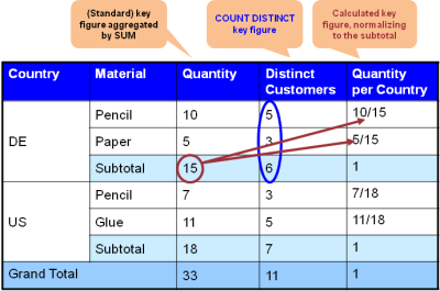
Let's look at an example which looks as if it was of "hello world style" but which quickly reveals some challenges. In figure 1, a standard OLAP query result is displayed. 

It shows the quantities of sold items per product and country. In addition, the number of distinct customers who bought those products can be seen. Finally, the quantity relative to the overall number of sold products in a country are presented as percentages.

Figure 1: Example of a result of an OLAP query

Some Challenges in the Example

Now when you carefully look at the example of figure 1 then you see some of the challenges: 

The numbers of distinct customers do not sum up. There are 5 distinct customers buying pencils and 3 buying paper, both in Germany (DE), but only 6 – and not 5+3=8 – buying products in DE. There must be 2 customers that have bought both, pencils and paper. In processing terms this means that the subtotal (e.g. by country) cannot be calculated out of the preceeding aggregation level (e.g. by country and product) but needs to be calculated from the lowest granularity (i.e. by country, product, customer). The calculated key figure quantity per country refers to the key figure quantity and sets the latter's values in relation to its subtotals. This means that the quantity key figure and its subtotals has to be calculated prior to calculating key figure quantity per country. This means there is an order of processing imposed by mathematics.

Figure 2: Challenges in the example

What you can do with SQL

In order to calculate the result of figure 1, classic BW (or SQL-based OLAP tools in general) would issue a SQL statement that retrieves a rows similar to the one shown in figure 3. That row constitutes the base set of data from which the result of figure 1 can be calculated. It is not the final result yet but from that data it is possible to calculate the final result as indicated in figure 1. Don't get fooled by the small amount of data shown in figure 3, As you can see, it is necessary to get the details on the customers in order to calculate the distinct customers per group-by level. In real world scenarios – just imagine retailers, mobile phone or utility companies – the customer dimension can be huge, i.e. holding millions of entries. Consequently and caused by real-world combination, the result of the SQL query in figure 3 is likely to be huge in such cases. That "sub-result" needs to be further processed, traditionally in an application server, e.g. BW's ABAP server or the Web-intelligence server. This implies that huge amounts of data have to be transported from the DB server to such an application server or a client tool. 

Figure 3: Rowset retrieved by a SQL query to calculate result of figure 1

By the way: BWA 7.0 accelerated exactly this part of OLAP query processing, i.e. the basic data query. Subsequent processing on top has still been executed in the application server. This is not a big issue as long as the OLAP query is dominated by the SQL processing. However, it comes short - as in this example - when the result of the basic SQL query gets huge and requires significant data transport from the DB to the application server and then significant data traversals to calculate the final result. 

The "OLAP Calculation Graph"

Now based on the result shown in figure 3 there is a natural sequence of how to calculate the various formulas (behind the calculated key figures) and the various group aggregations (i.e. the subtotals and totals). 

Many of those subsequent calculations can be considered as SQL queries on top of figure 3's result. Figure 4 shows the resulting dependency graph: LQ is the label for the query of figure 3; L1, L2, ..., L6 are "queries" or calculations on top. BW's OLAP compiler basically derives that graph and sends it down to HANA's optimizer (using a proprietary interface), HANA optimizes and processes that graph and sends back the result. Please beware that the result is not a rowset, at least not in the normal sense. It is heterogeneous sets of rows that are returned and that need to go into the appropriate result line in figure 1. In short: the compiler creates a graph to be sent to HANA and then there is a postprocessing step that receives the result and converts it to the desired result set of the OLAP query (i.e. a cellset as in fig. 1). 

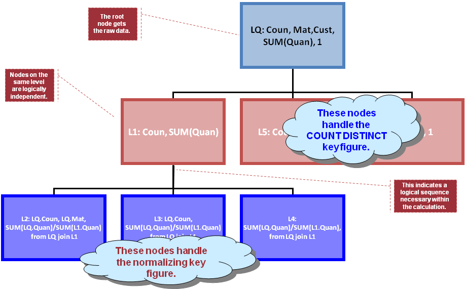
Figure 4: Graph derived for processing the final result (as in fig. 1) from the data in fig. 3

Concluding Remarks

Author think there is a few fundamental things that become apparent even by looking at the simple example discussed in this blog: Even though individual processing steps can be expressed via SQL, it is in the end a well defined sequence of processing steps that yield the result.

Accelerating the individual steps helps but falls short. For example, an OLAP client tool can derive an OLAP graph like the one in fig. 4. One alternative is that it issues for each node in that graph a SQL or SQL-like query. To avoid the data transport, it can materialize intermediate results. However, this constitutes an overhead. As a second alternative (the one frequently met in practice), it is possible to issue only the basic query - labeled "LQ" in fig. 4 - and transport a potentially huge result set over the network to the client in order to calculate the rest on the client level. This is the traditional approach which obviously also suffers from the transportation overhead.

BW-on-HANA resolves those issues by providing a powerful option to define an OLAP query - i.e. the BEx query - this is a precondition to allow all of that in the first place, sending down the entire processing graph to HANA and allowing HANA to optimize and pipeline the individual processing steps, and

having the capability to assemble the partial results of the processing steps into the final (OLAP) result.

Credits

Let me emphasize that I'm the mere republisher of this blog. The real credits go to the real author and bright minds behind this approach who sit in BW's OLAP and data manager teams.This blog is cross-published here. You can follow the author on Twitter via @tfxz.

Store locations from SAP BW to Google Maps

Store locations from SAP BW to Google Maps

via Content in SCN

There are times when we do something for one pure and simple reason: "Because We Can". So when Wally wanted to see all the customer stores in the country in Google maps, I said why not!

We can maintain a master data with the coordinates (latitude, longitude) in SAP BW and write a code which will read these coordinate from the master-data table and generate a geoRSS or a KML or a KMZ file.

There is a growing trend among internet users to use these file formats to exchange publish and consume geographical data, and moreover google maps consume them readily. These formats are more or less like a normal xml file with a few extra tags, that's all…

The only question in my mind was whether I could generate the KML file or not; but there is no reason why we can't considering that we can quite easily generate a XML.

So once we generate the KML through ABAP we can place it in share-point or some webhosting site and consume it directly though google maps.

It's cool for the customers to view their stores/plants in the map, and to know that they are indeed having a footprint in the information superhighway. 

In fact we can we can write a small app that will handle this in a more sophisticated manner in an Iphone.

How to use OpenDocument with BEx variables

How to use OpenDocument with BEx variables 

By Victor Gabriel Saiz Castillo

While the official OpenDocument guide is a great resource and explains in detail how to use OpenDocument syntax, We have not seen a good documentation explaining how to use OpenDocument in conjunction with SAP BW BEx variables, and yes, there are syntax differences depending on the different BEx variable types. 

What is the OpenDocument interface?

The OpenDocument interface allows you to open reports that are saved in the BI LaunchPad by using URL hyperlinks. You can take advantage of the OpenDocument syntax and parameterize the report to be opened.

How to pass values to BEx variables in general?

As everything in SAP BW, there is always a Text and a Key for every record in your report. The text is clearly not unique though, it depends for example on the language of the user that is currently viewing the report. On the other side most of the users are not very comfortable seeing and working only with technical keys, you should always pass both: Key and Text.

How do I construct an OpenDocument URL in general? 

While you can construct your own URL manually by carefully reading the manual, there is much fancier way: Use the hyperlink wizard! The hyperlink wizard is available only in Web Intelligence Web Mode (DHTML), it is not available in RIA mode (Java) nor in the Rich Client. You can open the hyperlink wizard by right-clicking on a field > Linking > Add Document Link:

After you select a target document in the hyperlink wizard, you will be presented with all the prompts of the target report. In this example I have a prompt (from a BEx variable) on a dimension object named "Material", an example of a material is a material named "Ten" with key "010". The following would be a correct way of passing a single material by using the dimension objects in a table:

In the first box you should provide a Text (Dimension Object), and in the second its corresponding key. In the screenshot above "Z_SINGLE_OPT_TEXT" corresponds to the description of the BEx variable, on the other side, the generated hyperlink will use the technical name of the variable.

How do I pass Single Values?

If you use the hyperlink wizard to pass a single value variable, you will notice that the wizard will use two parameters lsS for the Text and lsI for the key. If for example you click on a material "Ten" with key "010" using a variable "Z_SINGLE_OPT" (technical name):

You will get a syntax like this: 

"…lsSZ_SINGLE_OPT=Ten&lsIZ_SINGLE_OPT=010"

Notice that code is hard coded with the values for a better understanding, but of course you can use dimensions here.

How do I pass Multiple Single Values?

By separating individual values with a semicolon (;), you can pass multiple single values at a time. For example:

The corresponding syntax equates to: 

"…&lsMZ_MSV_OPT=Ten;Fourty&lsIZ_MSV_OPT=010;040"

Notice that lsM is used to pass multiple single values.

How do I pass Ranges?

When passing ranges you must separate the minimum and maximum value with two consecutive dots (..). The start and end of the range must have square brackets that you have to create manually:

Generated syntax: 

"…lsRZ_RANGE_OPT=[Ten..Thirty]&lsIZ_RANGE_OPT=[010..030]"

Notice that lsR will be used to pass ranges.

How do I pass nodes of a Hierarchy?

Passing a hierarchy node with standard text and key objects works fine most of the times, however I use following syntax (according to note 1677950) to avoid potential issues: [Hierarchy].key

In this case you will notice that a "0HIER_NODE/" will be inserted to all non-leaves in the hierarchy.

Generated syntax:
„…&lsSZ_HIER_OPT=Even&lsIZ_HIER_OPT=0HIER_NODE/EVEN"

How do I pass compounded objects?
In this case you need to make sure that the key that you are passing is not compounded (more Information in this blog post). You can achieve this by using formulas in the front-end e.g. "=right()" or by selecting the non-compounded key available since BI4 SP05:

Hope you enjoyed this introduction into using OpenDocument with BEx variables

Original Article of : Victor Gabriel Saiz Castillo

SAP BEX Toolbar

SAP BEX Toolbar - Ready Reckoner

Raj Salecha 

Create an InfoCube

Create an InfoCube

via Content in SCN

Creating an InfoCubeIn BW,Customer ID,Material Number,Sales Representative ID,Unit of Measure,and Transaction Date are called characteristics. Customer Name and Customer Address are attributes of Customer ID,although they are characteristics as well. Per Unit Sales Price,Quantity Sold,and Sales Revenue are referred to as key figures. Characteristics and key figures are collectively termed InfoObjects.

A key figure can be an attribute of a characteristic. For instance,Per Unit Sales Price can be an attribute of Material Number. In our examples,Per Unit Sales Price is a fact table key figure. In the real world,such decisions are made during the data warehouse design phase. InfoCube Design provides some guidelines for making such decisions.

InfoObjects are analogous to bricks. We use these objects to build InfoCubes. An InfoCube comprises the fact table and its associated dimension tables in a star schema.

In this chapter,we will demonstrate how to create an InfoCube that implements the star schema from figure. We start from creating an InfoArea. An InfoArea is analogous to a construction site,on which we build InfoCubes.

Creating an InfoArea

In BW,InfoAreas are the branches and nodes of a tree structure. InfoCubes are listed under the branches and nodes. The relationship of InfoAreas to InfoCubes in BW resembles the relationship of directories to files in an operating system. Let's create an InfoArea first,before constructing the InfoCube.

Work Instructions
Step 1. After logging on to the BW system,run transaction RSA1,or double-click Administrator Workbench.



Step 2. In the new window,click Data targets under Modelling in the left panel. In the right panel,right-click InfoObjects and select Create InfoArea….


Note
In BW,InfoCubes and ODS Objects are collectively called data targets.
Step 3. Enter a name and a description for the InfoArea,and then mark to continue.


Result
The InfoArea has been created.

Creating InfoObject Catalogs
Before we can create an InfoCube,we must have InfoObjects. Before we can create InfoObjects,however,we must have InfoObject Catalogs. Because characteristics and key figures are different types of objects,we organize them within their own separate folders,which are called InfoObject Catalogs. Like InfoCubes,InfoObject Catalogs are listed under InfoAreas.

Having created an InfoArea,let's now create InfoObject Catalogs to hold characteristics and key figures.

Work Instructions
Step 1. Click InfoObjects under Modelling in the left panel. In the right panel,right-click InfoArea–demo,and select Create InfoObject catalog….
Step 2. Enter a name and a description for the InfoObject Catalog,select the option Char.,and then click to create the InfoObject Catalog.
Step 3. In the new window,click to check the Info Object Catalog. If it is valid,click to activate the InfoObject Catalog. Once the activation process is finished,the status message InfoObject catalog IOC_DEMO_CH activated appears at the bottom of the screen.


Result
Click to return to the previous screen. The newly created InfoObject Catalog will be displayed,as shown in Screen

Following the same procedure,we create an InfoObject Catalog to hold key figures. This time,make sure that the option Key figure is selected Screen.

Creating InfoObjects-Characteristics

Now we are ready to create characteristics.

Work Instructions
Step 1. Right-click InfoObject Catalog–demo: characteristics,and then select Create InfoObject….

Step 2. Enter a name and a description,and then click to continue.

Step 3. Select CHAR as the DataType,enter 15 for the field Length,and then click the tab Attributes.

Step 4. Enter an attribute name IO_MATNM,and then click to create the attribute.

Note: Notice that IO_MATNM is underlined. In BW,the underline works like a hyperlink. After IO_MATNM is created,when you click IO_MATNM,the hyperlink will lead you to IO_MATNM's detail definition window.
Step 5. Select the option Create attribute as characteristic,and then click to continue.


Step 6. Select CHAR as the DataType,and then enter 30 for the field Length. Notice that the option Exclusively attribute is selected by default. Click to continue.

Note: If Exclusively attribute is selected,the attribute IO_MATNM can be used only as adisplay attribute,not as a navigational attribute. "InfoCube Design Alternative I Time Dependent Navigational Attributes," discusses an example of the navigation attributes.

Selecting Exclusively attribute allows you to select Lowercase letters. If the option Lowercase letters is selected,the attribute can accept lowercase letters in data to be loaded.

If the option Lowercase letters is selected,no master data tables,text tables,or another level of attributes underneath are allowed. "BW Star Schema," describes master data tables and text tables,and explains how they relate to a characteristic.
Step 7. Click to check the characteristic. If it is valid,click to activate the characteristic.

Step 8. A window is displayed asking whether you want to activate dependent InfoObjects. In our example,the dependent InfoObject is IO_MATNM.

Click to activate IO_MAT and IO_MATNM.


Result
You have now created the characteristic IO_MAT and its attribute IO_MATNM.

Note: Saving an InfoObject means saving its properties,or meta-data. You have not yet created its physical database objects,such as tables.

Activating an InfoObject will create the relevant database objects. After activating IO_MAT,the names of the newly created master data table and text table are displayed under the Master data/texts tab. The name of the master data table is /BIC/PIO_MAT,and the name of the text table is /BIC/TIO_MAT.

Notice the prefix /BIC/ in the database object names. BW prefixes /BI0/ to the names of database objects of Business Content objects,and it prefixes /BIC/ to the names of database objects of customer-created BW objects.

Repeat the preceding steps to create the other characteristics listed.
CHARACTERISTICS


The column "Assigned to" specifies the characteristic to which an attribute is assigned. For example,IO_MATNM is an attribute of IO_MAT.

The Material Description in Table will be treated as IO_MAT's text,as shown in Table,"Creating InfoPackages to Load Characteristic Data." We do not need to create a characteristic for it.

IO_SREG and IO_SOFF are created as independent characteristics,instead of IO_SREP's attributes. Section 3.6,"Entering the Master Data,Text,and Hierarchy Manually," explains how to link IO_SOFF and IO_SREG to IO_SREP via a sales organization hierarchy. "InfoCube Design Alternative I—Time-Dependent Navigational Attributes," discusses a new InfoCube design in which IO_SOFF and IO_SREG are IO_SREP's attributes.

BW provides characteristics for units of measure and time. We do not need to create them.From Administrator Workbench,we can verify that the characteristics in Table have been created by clicking InfoArea–demo,and then clicking InfoObject Catalog–demo: characteristics.


Creating Info Objects-Key Figures

Next,we start to create the keys.

Work Instructions
Step 1. Right-click InfoObject Catalog–demo: key figures,and then select Create InfoObject.
Step 2. Enter a name and a description,and then click to continue.
Step 3. Select Amount in the block Type/data type,select USD as the Fixed currency in the block Currency/unit of measure,and then click to check the key figure. If it is valid,click to activate the key figure.

Result
You have created the key figure IO_PRC. A status message All InfoObject(s) activated will appear at the bottom of Screen.

Repeat the preceding steps to create other key figures listed.
KEY FIGURES


From Administrator Workbench,we can verify that the key figures in Table have been created (Screen) by clicking InfoArea–demo,and then clicking InfoObject Catalog–demo: key figures.

Having created the necessary InfoObjects,we now continue to create the InfoCube.

Creating an InfoCube

The following steps demonstrate how to create an InfoCube,the fact table and associated dimension tables,for the sales data shown in Table

Work Instructions
Step 1. Select Data targets under Modelling in the left panel. In the right panel,right-click InfoArea–demo and then select Create InfoCube….

Step 2. Enter a name and a description,select the option Basic Cube in block InfoCube type,and then click to create the InfoCube.

Note: An InfoCube can be a basic cube,a multi-cube,an SAP remote cube,or a general remote cube.A basic cube has a fact table and associated dimension tables,and it contains data. We are building a basic cube.

A multi-cube is a union of multiple basic cubes and/or remote cubes to allow cross-subject analysis. It does not contain data. See,Aggregates and Multi-Cubes,for an example.

A remote cube does not contain data;instead,the data reside in the source system. A remote cube is analogous to a channel,allowing users to access the data using BEx. As a consequence,querying the data leads to poor performance.

If the source system is an SAP system,we need to select the option SAP RemoteCube. Otherwise,we need to select the option Gen. Remote Cube. This book will not discuss remote cubes.

Step 3. Select IO_CUST,IO_MAT,and IO_SREP from the Template table,and move them to the Structure table by clicking

Next,click the Dimensions… button to create dimensions and assign these characteristics to the dimensions.

Step 4. Click,and then enter a description for the dimension.

Note: BW automatically assigns technical names to each dimension with the format <InfoCube name><Number starting from 1>.

Fixed dimension <InfoCube name><P|T|U> is reserved for Data Packet,Time,and Unit. Section,"Data Load Requests," discusses the Data Packet dimension.

A dimension uses a key column in the fact table. In most databases,a table can have a maximum of 16 key columns. Therefore,BW mandates that an InfoCube can have a maximum of 16 dimensions: three are reserved for Data Packet,Time,and Unit; the remaining 13 are left for us to use.

Repeat the same procedure to create two other dimensions. Next,click the Assign tab to assign the characteristics to the dimensions.

Step 5. Select a characteristic in the Characteristics and assigned dimension block,select a dimension to which the characteristic will be assigned in the Dimensions block,and then click to assign the characteristic to the dimension.

Step 6. After assigning all three characteristics to their dimensions,click to continue.

Step 7. Select the Time characteristics tab,select 0CALDAY from the Template table,and move it to the Structure table by clicking

Step 8. Select the Key figures tab,select IO_PRC,IO_QUAN,and IO_REV from the Template table and move them to the Structure table by clicking.
Next,click to check the InfoCube. If it is valid,click to activate the InfoCube.

Result:
You have created the InfoCube IC_DEMOBC. A status message InfoCube IC_DEMOBC activated will appear at the bottom of Screen.

Summary

In this chapter,we created an InfoCube. To display its data model,you can right-click InfoCube–demo: Basic Cube,then select Display data model….

The data model appears in the right panel of Screen .

Note:
IO_SREG and IO_SOFF are not listed under IO_SREP as attributes; rather,they have been created as independent characteristics. "Entering the Master Data,Text,and Hierarchy Manually," describes how to link IO_SOFF and IO_SREG to IO_SREP via a sales organization hierarchy. "InfoCube Design Alternative I— Time-Dependent Navigational Attributes,"discusses a new InfoCube design in which IO_SOFF and IO_SREG are IO_SREP's attributes.

---END---